October 18, 2020

Oxygen Isotope Analysis in Paleoclimatology

October 18, 2020/ webmaster

The intent of this article is to provide a simplified explanation for the uses of oxygen isotope analysis in determining past climatic conditions. We’ve had several speakers over the last few years who have used or made reference to this type of analysis and so you might find this information helpful in understanding a future GSOC talk.

Most of us are familiar with the “solar system” type atomic model of oxygen from our K-12 education, having 8 electrons, 8 protons and 8 neutrons. In actuality, there are quite a few types of oxygen atoms out there, some containing as few as 3 neutrons and as many as 18 neutrons! Fortunately for scientists, only 3 of these oxygen isotopes are stable: the familiar ¹⁶O isotope; the 9-neutron type ¹⁷O; and the 10-neutron variety ¹⁸O. The others are radioactive and unstable. I’m going to be notationally lazy and call these O16, or “light” oxygen, O17, and O18, or “heavy” oxygen.

99.762% of the oxygen found in earth’s atmosphere is O16 and 0.204% is O18. O17 comes in a distant third in abundance at 0.037%, and is generally not studied in these analyses. Since they are stable, at any time the earth contains a finite number of these isotopes and we’ll be looking at how they are distributed in atmospheric water, surface water, and the oceans. This analysis is a type of shell game for any given climatic condition and global climate is the primary factor in variations of O18 abundance in any one location, although other factors come to play in analyzing samples and determining past climate temperatures.

The core observation driving the model used in paleoclimate analysis of oxygen isotopes is that heavy oxygen is less likely to evaporate than light oxygen. That is, it takes relatively more energy for a water molecule containing a heavy oxygen isotope to evaporate, and this effect is more pronounced the lower the temperature of the atmosphere. The scientific term for this effect is fractionation, a process of concentrating certain types of matter (in this case isotopes) in response to a phase change.

The abundance of heavy oxygen in comparison to light oxygen is measured in a unit called δ¹⁸O (delta O-eighteen), calculated from the following formula:

The standard ratio is based on a value called Vienna Standard Mean Ocean Water (VSMOW) where O18 to O16 is 0.020052 -- this is an arbitrary value selected by an international standard agreement. The unit symbol ‰ refers to parts per 1000 and is called a “per mille” symbol. Using this formula, we characterize an overabundance of O18 with a positive δ¹⁸O value and a dearth of O18 with a negative δ¹⁸O value.

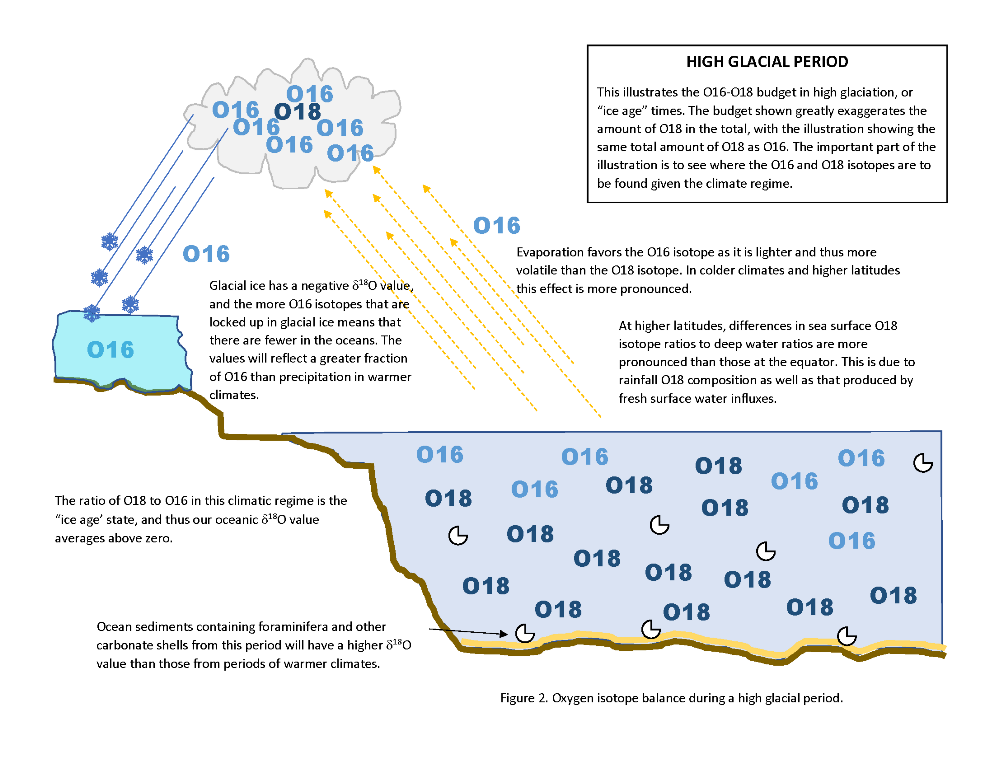
Looking at Figures 1 and 2 above (click on them to enlarge), we see that the fractionation of O18 is more pronounced in colder conditions than in warmer “normal” conditions. This means that in colder conditions evaporated water has more O16 than in warmer conditions. The opposite is true for oceans during colder conditions – there we find a higher concentration of O18 in colder than in warmer conditions. So when we are looking for evidence of past paleoclimates, it matters where and what we are sampling as to how the data is analyzed.

A common proxy used in the analysis of past climates is by measuring δ¹⁸O in the carbonate shells of foraminifera and other carbonate shelled animals that collect in ocean floor sediments. When these creatures die the shells fall to the sea floor. Because the sediments come from animals living in the ocean, higher δ¹⁸O values indicate a colder past climate and lower δ¹⁸O values indicate a warmer past climate. Analysis may also be species, and even size-specific for data consistency.

Conversely, if the samples are ice taken from glacier cores, lower δ¹⁸O values indicate a colder past climate and higher δ¹⁸O values indicate a warmer past climate. This is because the glacier ice lies on the other end of the evaporation cycle described in Figures 1 and 2 above.

Ok, now that we’ve gotten the basic principles down, what do these oxygen isotope analyses show for past climates? Here are examples of paleoclimatology for the Pliocene/Pleistocene to modern times, and the Cenozoic era.

The first example comes from data obtained in a 2005 (Lisiecki and Raymo) study and is the product of stacking 57 foraminifera records from seafloor sediment cores around the world together, which averages the values and decreases the influence of ocean currents and other local anomalies. The record serves to confirm the timeline for the beginning of the Pleistocene ice age. It also has a pattern of cycles which do correspond to astronomical data for the earth’s orbit and wobble (Milankovitch cycles). The right-side scale refers to the δ¹⁸O values taken in the 2005 stacked records. The scale on the left is the corresponding temperatures derived from the δ¹⁸O values in ice cores for 420 ka taken in Vostok Station, Antarctica, in the 1970’s.

The second example comes from a study done with a larger scope of time as its target. This study was based on data from the Deep Sea Drilling Project (1968-1983). Here we see a very amazing account of the past temperatures during the Cenozoic record. Earth’s oceanic temperatures have varied quite a lot. During the Eocene epoch, for example, Antarctica was not frozen as it is today, and temperatures everywhere were quite a bit warmer. All this data gives climate scientists a way to look at the past and also a lens from which to view the future.

Citations for illustrations used in this article:

Pages used to collect illustrations with references to data origins: https://commons.wikimedia.org/wiki/File:Five_Myr_Climate_Change.png, https://commons.wikimedia.org/wiki/File:65_Myr_Climate_Change.png and https://en.wikipedia.org/wiki/Vostok_Station#Ice_core_drilling.

Citation for 65 Ma data illustration: CC BY-SA 3.0

Citation for 5.5 Ma data illustration: By Dragons flight (Robert A. Rohde) - original image by User:Dragons flight, based on data (figure 4?) from Lisiecki and Raymo (2005), CC BY-SA 3.0

References and Additional Reading:

R. Dorsey, “A Brief Explanation of Oxygen Isotopes in Paleoclimate studies”

Lisiecki, L. E., and M. E. Raymo (2005), “A Pliocene-Pleistocene stack of 57 globally distributed benthic δ18O records,” Paleoceanography, 20, PA1003, doi:10.1029/2004PA001071.

Zachos, James, Mark Pagani, Lisa Sloan, Ellen Thomas, and Katharina Billups (2001). "Trends, Rhythms, and Aberrations in Global Climate 65 Ma to Present". Science 292 (5517): 686–693. doi:10.1126/science.1059412.

Zachos, James C; Stott, Lowell D; Lohmann, Kyger C (1994): “Stable isotope ratios of foraminifera from various DSDP/ODP sites.” PANGAEA, https://doi.org/10.1594/PANGAEA.729901, supplement to: Zachos, JC et al. (1994): Evolution of early Cenozoic marine temperatures. Paleoceanography, 9(2), 353-387,

Wikipedia articles “Isotopes of oxygen” and “δ18O.”

Synopsis of the Deep Sea Drilling Project: 50 Years of Ocean Discovery: National Science Foundation 1950-2000, Ocean Studies Board, National Research Council, ISBN: 0-309-51744-3, 276 pages, 8.5 x 11, (2000), pp. 59-61,124-125.

NASA Earth Observatory Website has a good explanation of paleoclimatology and its relationship to Earth’s orbit (Milankovitch cycles).

Harvard University’s page on Equable Climate evidence

Ana Christina Ravelo! and Claude Hillaire-Marcel, “The Use of Oxygen and Carbon Isotopes of Foraminifera in Paleoceanography,” Chapter 18, Developments in Marine Geology, Volume 1 r 2007 Elsevier B.V., ISSN 1572-5480, DOI 10.1016/S1572-5480(07)01023-8.

Videos:

Minute Earth, “How These Sea Shells Know the Weather in Greenland,” A really fun You Tube video!

Callan Bentley, “An introduction to isotope fractionation,” You Tube video containing simple explanations for isotope fractionation.

A longer but very worthwhile video from The Geological Society London Lecture Series of 2015 features University of Cambridge professor Colin Summerhayes’ lecture “Earth’s Climate Evolution.” The lecture reviews the history of climate research in tandem with development of plate tectonics and other key geological developments to future climatic predictions. It is well-produced and easy to hear and has some great slides.

Are you planning your career and interested in this dance between life and climate and geology? Check out this video about the emerging multidisciplinary field of biogeodynamics.

Featured